OutflowModel
-
class
sf3dmodels.outflow.OutflowModel(pos_c, axis, z_min, z_max, dx)[source] [edit on github]¶ Bases:
sf3dmodels.outflow.core.RandomGridHost class for outflow models. The grid points are generated randomly taking into account the Jet model geometry.
Available models:
- ‘reynolds86’: Jet Model (Reynolds+1986)
Input units: SI (metres, kilograms, seconds).
Parameters: - pos_c : array_like, shape (3,)
Origin of coordinates on the axis.
- axis : array_like, shape (3,)
Long axis direction, of arbitrary length. For example, an axis pointing to the z-direction: axis = [0,0,1]
- z_min : scalar
Axis lower limit to compute the physical properties.
- z_max : scalar
Axis upper limit to compute the physical properties. The axis extent will be [z_min, z_max].
- dx : scalar
Maximum separation between two adjacent grid points. This will prevent void holes when merging this random grid into a regular grid of nodes separation = dx.
- mirror : bool, optional
If True, it is assumed that the model is symmetric to the reference position
pos_c. Defaults to True.
Methods Summary
reynolds86(self, width_pars[, dens_pars, …])Outflow Model from Reynolds+1986. Methods Documentation
-
reynolds86(self, width_pars, dens_pars=None, ionfrac_pars=None, temp_pars=None, v0=None, abund_pars=None, gtdratio=None, vsys=[0, 0, 0], z0=None)[source] [edit on github]¶ Outflow Model from Reynolds+1986.
- See the Table 1 on Reynolds+1986 for examples on the combination of parameters and their physical interpretation.
- See the model equations and a sketch of the jet geometry in the Notes section below.
- The resulting Attributes depend on which parameters were set different to None.
Input and output units: SI (metres, kilograms, seconds).
Parameters: - width_pars : array_like, shape (2,)
[\(w_0\), \(\epsilon\)]: parameters to compute the Jet half-width at each \(z\).
- dens_pars : array_like, shape (2,)
[\(n_0\), \(q_n\)]: parameters to compute the Jet number density.
- ionfrac_pars : array_like, shape (2,)
[\(x_0\), \(q_x\)]: parameters to compute the ionized fraction of gas.
- temp_pars : array_like, shape (2,)
[\(T_0\), \(q_T\)]: parameters to compute the Jet temperature.
- abund_pars : array_like, shape (2,)
[\(a_0\), \(q_a\)]: parameters to compute the molecular abundance.
- z0 : scalar
Normalization distance. Must be different to 0 (zero) to avoid divergences.
If None,
z_max/100is used.Defaults to None.
- v0 : scalar
Gas speed at
z0. Speed normalization factor. For mass conservation: \(q_v=-q_n-2\epsilon\).- gtdratio : scalar
Gas-to-dust ratio value (mass ratio). Uniform at every point of the grid.
- vsys : array_like, shape (3,)
[\(v_{0x}, v_{0y}, v_{0z}\)]: Systemic velocity to be added to the final Jet velocity field.
Defaults to [0,0,0].
Notes
Model equations:
With \(r = \sqrt{x^2 + y^2+ z^2}\),\[ \begin{align}\begin{aligned}w(z) &= w_0(z/z_0)^\epsilon \\n_{H}(z) &= n_0(z/z_0)^{q_n} \\T(z) &= T_0(z/z_0)^{q_T} \\x(z) &= x_0(z/z_0)^{q_x} \\n_{ion}(z) &= n_{H}(z) x(z)\\a(z) &= a_0(z/z_0)^{q_a} \\v(z) &= v_0(z/z_0)^{q_v} \\\vec{v}(r) &= v(z) \hat{r}, \end{aligned}\end{align} \]where \(q_v = -q_n-2\epsilon\) for mass conservation.
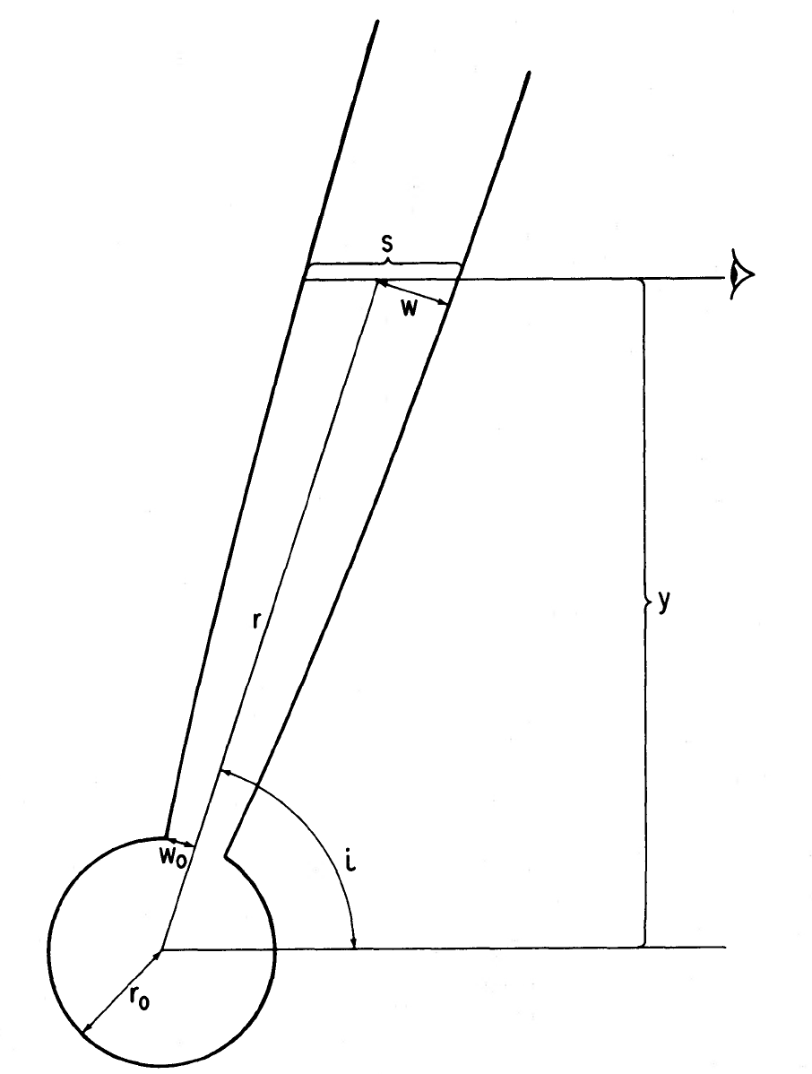
Figure 1 from Reynolds+1986. Jet geometry. Note that the \(r\) from the sketch is \(z\) in our equations.
Examples
Have a look at the examples/outflows/ folder on the GitHub repository.
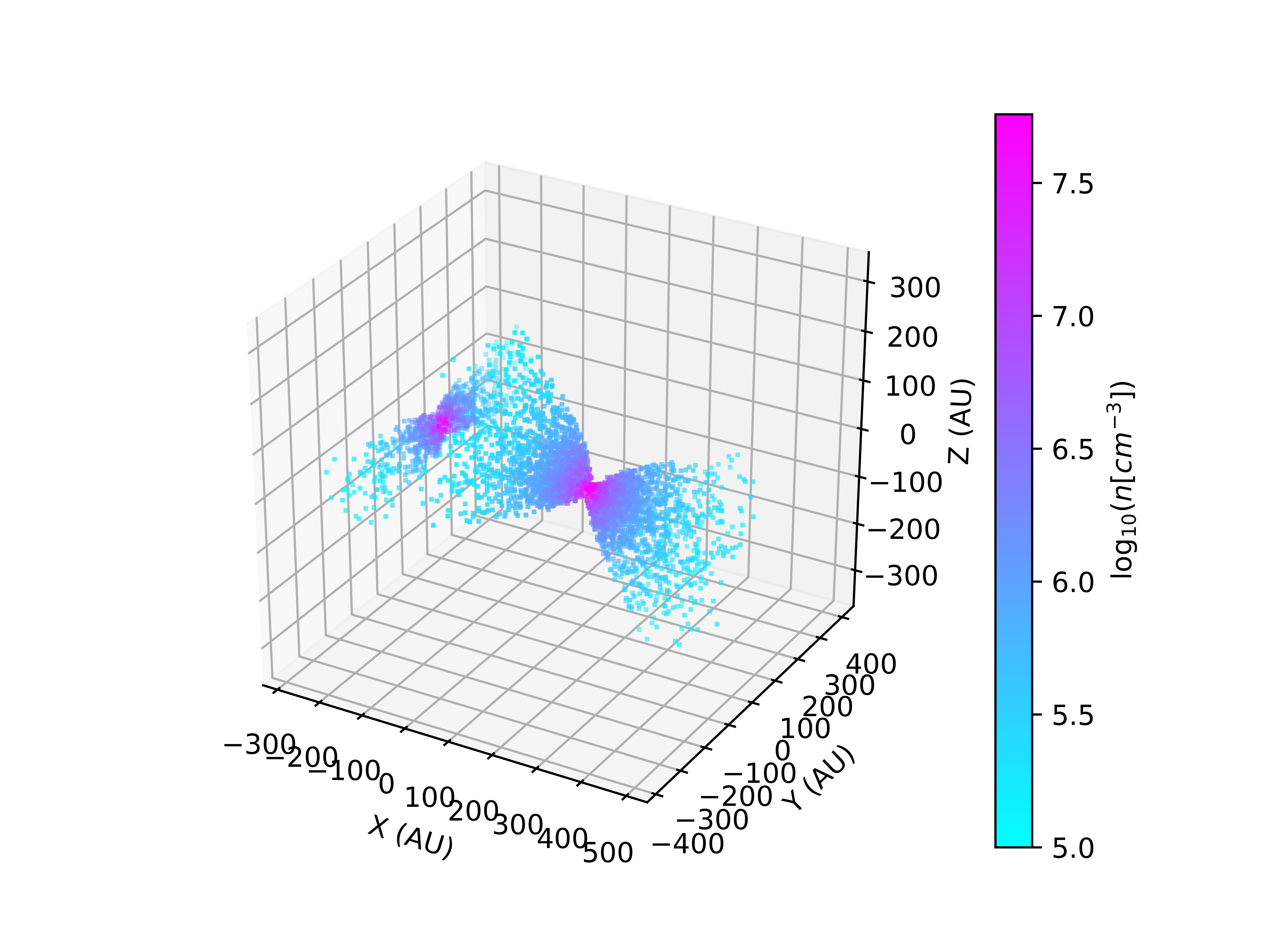
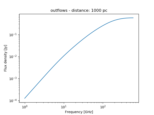
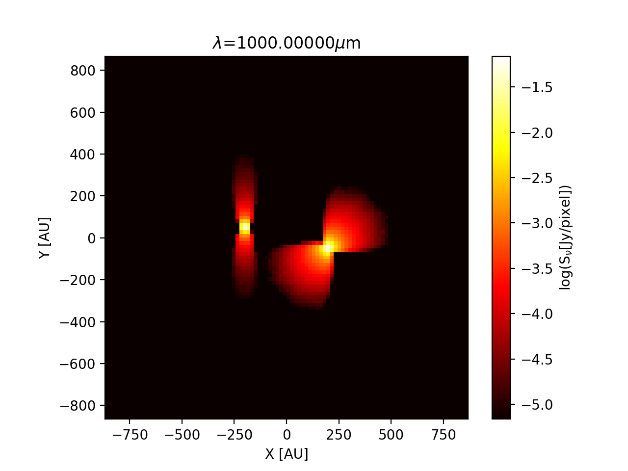
The example there shows how to compute the free-free emission from a couple of outflows using RADMC-3D. Figures below, from left to right: Grid points distribution and their density; Spectral Energy Distribution; Free-free continuum image at \(\lambda=\) 1000 microns.
Attributes: - density :
numpy.ndarray, shape (n,) Atomic hydrogen number density.
- temperature :
numpy.ndarray, shape (n,) Gas temperature.
- ionfraction :
numpy.ndarray, shape (n,) Ionized fraction of hydrogen.
- density_ion :
numpy.ndarray, shape (n,) Ionized hydrogen number density: density * ionfraction.
- speed :
numpy.ndarray, shape (n,) Speed.
- vel :
Struct, The velocity field. Attributes: vel.x, vel.y, vel.z, shape (n, ) each.
- abundance :
numpy.ndarray, shape (n,) Molecular abundance.
- gtdratio :
numpy.ndarray, shape (n,) Gas-to-dust ratio.
- GRID :
Struct, Grid point coordinates and number of grid points.
Attributes: GRID.XYZ, shape(3,n): [x,y,z]; GRID.NPoints, scalar.
- r :
numpy.ndarray, shape (n,) Grid points distance to the outflow centre.