FilamentModel

class sf3dmodels.filament.FilamentModel(pos_c, axis, z_min, z_max, dx, mirror=False)

Bases: sf3dmodels.grid.RandomGridAroundAxis, sf3dmodels.filament.DefaultFilamentFunctions

Host class for filament models.

The grid points are generated randomly taking into account the filament width as a function of the Z-coordinate.

Available models:

• Smith+2014b: See the model functions on DefaultFilamentFunctions

Input units: SI (metres, kilograms, seconds).

Parameters:

pos_c : array_like, shape (3,)

Origin of coordinates on the axis.

axis : array_like, shape (3,)

Long axis direction, of arbitrary length. For example, an axis pointing to the z-direction: axis = [0,0,1]

z_min : scalar

Axis lower limit to compute the physical properties.

z_max : scalar

Axis upper limit to compute the physical properties. The axis extent will be [z_min, z_max].

dx : scalar

Maximum separation between two adjacent grid points. This will prevent void holes when merging this random grid into a regular grid of nodes separation = dx.

mirror : bool, optional

If True, it is assumed that the model is symmetric to the reference position pos_c. Defaults to False.

Notes

The reference axis to compute \(\theta\) is gotten as follows:

>>> cart = np.zeros(3) #Initialise an empty cartesian vector.
>>> cart[np.argmin(axis)] = 1. #Make 1 the component where the axis vector is shorter. 
>>> axis_theta = np.cross(axis, cart) #The reference axis for theta is the cross product of axis and cart.

Methods Summary

cylinder(self, width_pars, R_min[, …])

Filament Model from Smith+2014b.

Methods Documentation

cylinder(self, width_pars, R_min, dens_pars=[10000000000.0, 3085677581489926.0, 1.0], temp_pars=[100.0, 308567758148992.6, -0.5], vel_pars=[(1000.0, 308567758148992.6, -0.5), 500.0, 800.0], abund_pars=1e-08, gtdratio_pars=100.0, vsys=[0, 0, 0], dummy_frac=0.0, dummy_values={'abundance': 1e-12, 'temperature': 2.72548, 'density': 1000.0, 'gtdratio': 100.0, 'vx': 0.0, 'vy': 0.0, 'vz': 0.0})

Filament Model from Smith+2014b.

• See Section 2.4 and Tables 2,5 and 6 of Smith+2014b for examples on different combination of parameters.
• See the model equations and a sketch of the cylinder geometry in the Notes section below.
• See the model functions on DefaultFilamentFunctions.
• It is possible to customise the model functions in order to control the filament geometry, density, etc. See the example section below.
• The object Attributes depend on which physical parameters were set different to None.

Input and output units: SI (metres, kilograms, seconds).

Parameters:

width_pars : scalar or array_like, shape (npars,)

Parameters to compute the filament half-width at each \(z\).

Expecting: \(w_0\)

R_min : scalar,

Minimum radius from the long axis to compute the physical properties.

Must be different to zero to avoid divergences in the model functions.

dens_pars : scalar or array_like, shape (npars,)

Parameters to compute the filament number density.

Expecting: [\(n_c\), \(R_{\rm flat}\), \(p\)]

Default values: [1e10, 0.1pc, 1.0]

temp_pars : scalar or array_like, shape (npars,)

Parameters to compute the filament temperature.

Expecting: [\(T_0\), \(R_0\), \(p\)]

Default values: [100., 0.01pc, -0.5]

vel_pars : scalar or array_like, shape (npars,)

Parameters to compute the filament temperature.

Expecting: [(\(v_{\small{\rm R_0}}\), \(R_0\), \(p\)), \(v_{\theta_0}\), \(v_{z_0}\)]

Default values: [(1000., 0.01pc, -0.5), 500., 800.]

abund_pars : scalar or array_like, shape (npars,)

Parameters to compute the filament molecular abundance.

Expecting: \(a_0\)

Default values: 1e-8

gtdratio_pars : scalar or array_like, shape (npars,)

Parameters to compute the filament gas-to-dust ratio.

Expecting: \(\rm{gtd}0\)

Default values: 100.

vsys : array_like, shape (3,)

[\(v_{0x}, v_{0y}, v_{0z}\)]: Systemic velocity to be added to the final cylinder velocity field.

Defaults to [0,0,0].

dummy_frac : scalar

Fraction of additional points (dummy points) to fill the grid borders. For radiative transfer purposes it is strongly recommended to set on this parameter (to at least 0.3) in case the width function of the filament is not constant, so that the RT code(s) can know explicitly where the empty spaces are and does not perform any kind of emission interpolation. Defaults to 0.0

ndummies = dummy_frac*npoints

dummy_values : dict

Dictionary containing the values of the properties of the dummy points. It will only be used if dummy_frac > 0.0

Raises:

ValueError : If R_min == 0.0

Warning

For radiative transfer purposes, if you modify the width function func_width it is strongly recommended to set on the dummy_frac parameter (to at least 0.3), so that the RT code(s) can know explicitily where the empty spaces are and does not perform any kind of emission interpolation.

Notes

Default model equations: DefaultFilamentFunctions

Figure 1. Sketches showing the basic input geometrical components that shape the filament. Left: edge-on view, Right: face-on view. The solid vectors and lengths are referred to the filament frame of reference and the dashed vectors to the GRID frame of reference.

Examples

Note

The source codes of the examples below can be found in the examples/outflows/ folder on the GitHub repository.

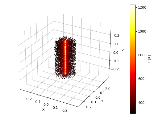
Let’s get started with the simplest model. The default filament is used except for the temperature and abundance parameters. It’s centred at (0,0,0); pointing to \(z\), i.e (0,0,1); with 0.4 pc of length and 0.1 pc of width.

import numpy as np
import sf3dmodels.filament as sf
import sf3dmodels.Plot_model as pm
from sf3dmodels.utils.units import pc

f1 = sf.FilamentModel([0,0,0], [0,0,1], -0.2*pc, 0.2*pc, 0.01*pc) # Instantiate the FilamentModel class with geometrical parameters for the grid construction
f1.cylinder(0.1*pc, 1e-3*pc, temp_pars = [500, 0.02*pc, -0.3], abund_pars = 1e-4) # Specify the method and the physical parameters

lims=np.array([-0.3,0.3])*pc

pm.scatter3D(f1.GRID, f1.density, np.mean(f1.density), axisunit = pc,
             colordim = f1.temperature,
             colorlabel = 'T [K]',
             xlim=lims, ylim=lims, zlim=lims,
             NRand = 10000, show=True)

(Source code, png, hires.png, pdf)

Figure 2. The plot shows 10000 grid points, randomly picked based on their density. The colours represent the temperature of the grid points.

For the radiative transfer we need to construct the prop dictionary and write the necessary files depending on the code that will be used (see Lime or Radmc3d):

import sf3dmodels.rt as rt
prop = {'dens_H': f1.density,
        'temp_gas': f1.temperature,
        'abundance': f1.abundance,
        'gtdratio': f1.gtdratio,
        'vel_x': f1.vel.x,
        'vel_y': f1.vel.y,
        'vel_z': f1.vel.z,
        }

lime = rt.Lime(f1.GRID)
lime.submodel(prop, output='datatab.dat', folder='./', 
              lime_header=True, lime_npoints=True)

Since the grid of our filament is non-regular the command to run Lime in sf3dmodels mode will have an additional -G flag:

$ lime -nSG -p 4 model.c

It will generate a set of cubes containing the \(^{12}\rm CO\) J=1-0 line emission and the dust emission for this model.

Figure 3. 115 GHz dust emission from the default cylindrical filament for two different orientations.

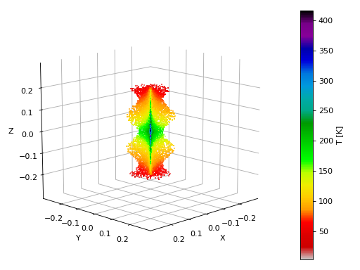
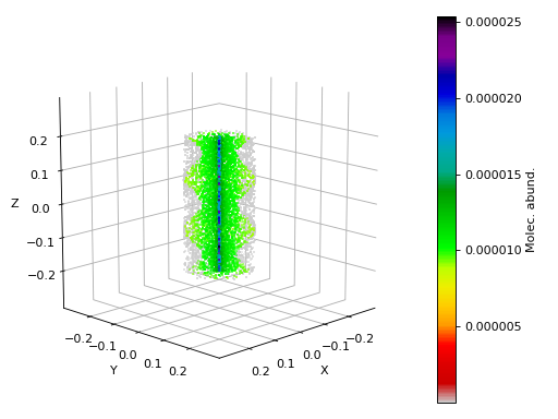
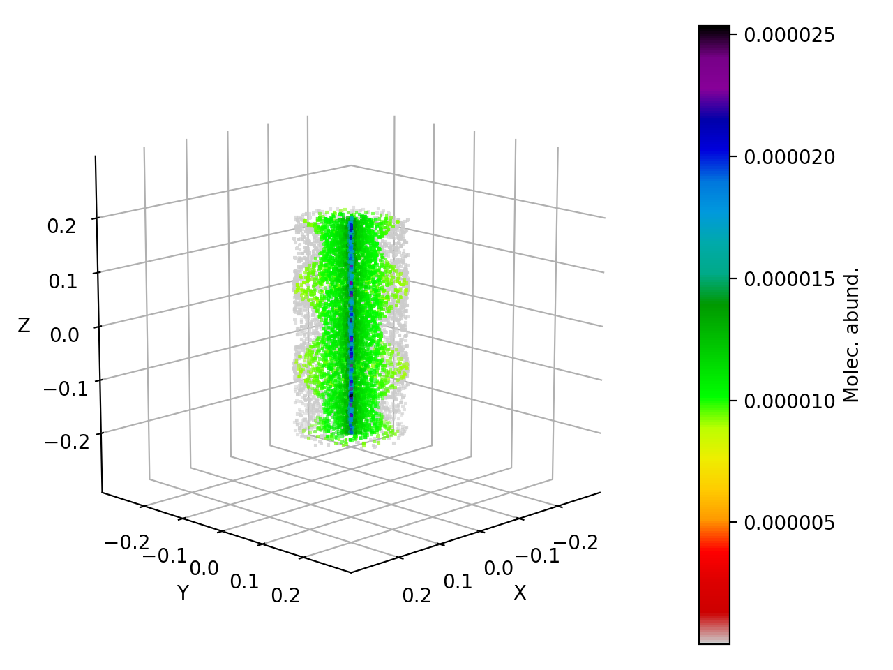
Let’s now customise some model functions and compute again the radiative transfer. This time the temperature will also be a function of \(z\), the abundance is no longer constant, and the width is a sine function of \(z\).

import numpy as np
import sf3dmodels.filament as sf
import sf3dmodels.Plot_model as pm
from sf3dmodels.utils.units import pc

f1 = sf.FilamentModel([0,0,0], [0,0,1], -0.2*pc, 0.2*pc, 8e-3*pc)

def new_width(z, *width_pars):
    w0, period = width_pars
    return w0*((0.5*np.sin(z*2*np.pi/period)**2) + 0.5)

def new_abund(R,theta,z, *abund_pars):
    a0, R0, p = abund_pars
    ca = a0*R0**-p
    return ca*R**p

def new_temp(R,theta,z, *temp_pars):
    TR, R0, pR, zh = temp_pars
    cR = TR*R0**-pR
    return cR*R**pR * np.exp(np.abs(z)/zh)

f1.func_width = new_width
f1.func_abund = new_abund
f1.func_temp = new_temp

f1.cylinder([0.1*pc, 0.3*pc], 1e-4*pc,
            abund_pars = [1e-5, 0.05*pc, -0.15],
            temp_pars = [200, 0.02*pc, -0.15, -0.17*pc],
            dummy_frac = 0.5)

lims=np.array([-0.3,0.3])*pc

pm.scatter3D(f1.GRID, f1.density, np.mean(f1.density), axisunit = pc,
             colordim = f1.temperature,
             colorlabel = 'T [K]',
             NRand = 10000,
             cmap = 'nipy_spectral_r',
             xlim=lims, ylim=lims, zlim=lims,
             azim=45, elev=15, show=True)

pm.scatter3D(f1.GRID, f1.density, np.min(f1.density), axisunit = pc,
             colordim = f1.abundance,
             colorlabel = 'Molec. abund.',
             NRand = 10000,
             cmap = 'nipy_spectral_r',
             xlim=lims, ylim=lims, zlim=lims,
             azim=45, elev=15, show=True)

(Source code)

(png, hires.png, pdf)

(png, hires.png, pdf)

Figure 4. 10000 grid points, randomly chosen according to their density. In the top plot the colours represent the temperature of the grid points and in the bottom one the abundance. For the bottom plot the weighting value was reduced in order to make the dummy points visible (in gray colour), which were activated here for radiative transfer purposes.

And the block concerning to the radiative transfer:

import sf3dmodels.rt as rt
prop = {'dens_H': f1.density,
        'temp_gas': f1.temperature,
        'abundance': f1.abundance,
        'gtdratio': f1.gtdratio,
        'vel_x': f1.vel.x,
        'vel_y': f1.vel.y,
        'vel_z': f1.vel.z,
        }

lime = rt.Lime(f1.GRID)
lime.submodel(prop, output='datatab.dat', folder='./', 
              lime_header=True, lime_npoints=True)

$ lime -nSG -p 4 model.c

The dust emission:

Figure 5. 115 GHz dust emission from the customised filament for two different orientations.

Finally let’s compute the first two moment maps of \(^{12}\rm CO J=1-0\) from the Lime’s output:

>>> from astropy.io import fits
>>> from astropy.wcs import WCS
>>> from spectral_cube import SpectralCube

>>> fn = 'img_custom_CO_J1-0_LTE_jypxl_edgeon.fits'
>>> hdu = fits.open(fn)[0]
>>> hdu.header['CUNIT3'] = 'm/s' 

>>> w = WCS(hdu.header)
>>> cube = SpectralCube(data=hdu.data.squeeze(), wcs=w.dropaxis(3))

>>> m0 = cube.moment(order=0) # Moment 0 (Jy/pxl m/s)
>>> m1 = cube.moment(order=1) # Moment 1 (m/s)
>>> m0.write('moment0_'+fn, overwrite=True)
>>> m1.write('moment1_'+fn, overwrite=True)

>>> fig, ax = plt.subplots(ncols=2, subplot_kw = {'projection': w.celestial}, figsize = (12,6))

>>> im0 = ax[0].imshow(m0.array, cmap='hot')
>>> im1 = ax[1].imshow(m1.array, cmap='nipy_spectral')           
>>> cb0 = fig.colorbar(im0, ax=ax[0], orientation='horizontal', format='%.2f', pad=0.1)
>>> cb1 = fig.colorbar(im1, ax=ax[1], orientation='horizontal', pad=0.1)
>>> ax[0].set_title('Moment 0 - edgeon', fontsize = 14)
>>> ax[1].set_title('Moment 1 - edgeon', fontsize = 14)
>>> cb0.set_label(r'Jy pxl$^{-1}$ m s$^{-1}$', fontsize = 14)
>>> cb1.set_label(r'm s$^{-1}$', fontsize = 14)

>>> plt.tight_layout(pad=2.0)
>>> fig.savefig('customfilament_moments_edgeon.png')

Note

You can also combine filaments with other kind of models to reproduce more complex scenarios. The following images result from a filament + envelope model:

Attributes:

density : numpy.ndarray, shape (n,)

Gas number density.

temperature : numpy.ndarray, shape (n,)

Gas temperature.

vel : Struct,

The velocity field. Attributes: vel.x, vel.y, vel.z, shape (n, ) each.

abundance : numpy.ndarray, shape (n,)

Molecular abundance.

gtdratio : numpy.ndarray, shape (n,)

Gas-to-dust ratio.

GRID : Struct,

Coordinates of the grid points and number of grid points.

Attributes: GRID.XYZ, shape(3,n): [x,y,z]; GRID.NPoints, scalar.

R : numpy.ndarray, shape (n,)

Radial distance of the grid points, referred to the filament frame of reference.

theta : numpy.ndarray, shape (n,)

Azimuthal coordinate of the grid points, referred to the filament frame of reference.

z : numpy.ndarray, shape (n,)

Height of the grid points, referred to the filament frame of reference.

R_dir : numpy.ndarray, shape (n,3)

Radial unit vector of the grid points, referred to the filament frame of reference.

theta_dir : numpy.ndarray, shape (n,3)

Azimuthal unit vector of the grid points, referred to the filament frame of reference.

z_dir : numpy.ndarray, shape (n,3)

Z unit vector of the grid points, referred to the filament frame of reference.