Modelling a single star forming region
Example 1
Source code and figures on GitHub: single_main
Note
W33A MM1-Main: The most massive compact source of the complex star forming region W33A MM1.
Model: Ulrich envelope + Pringle disc.
Useful references: Keto+2010, Galvan-Madrid+2010, Maud+2017, Izquierdo+2018
The preamble:
#------------------
#Import the package
#------------------
from sf3dmodels import Model, Plot_model
from sf3dmodels import Resolution as Res
import sf3dmodels.utils.units as u
import sf3dmodels.rt as rt
#-----------------
#Extra libraries
#-----------------
from matplotlib import colors
import numpy as np
import os
import time

t0 = time.time()
a. Let’s define some general parameters:
MStar = 7.0 * u.MSun
MRate = 4e-4 * u.MSun_yr #Mass accretion rate
RStar = 26 * u.RSun * ( MStar/u.MSun )**0.27 * ( MRate / (1e-3*u.MSun_yr) )**0.41
LStar = 3.2e4 * u.LSun
TStar = u.TSun * ( (LStar/u.LSun) / (RStar/u.RSun)**2 )**0.25
Rd = 152. * u.au #Centrifugal radius

print ('RStar:', RStar/u.RSun, ', LStar:', LStar/u.LSun, ', TStar:', TStar)
b. Create the grid that will host the region:
# Cubic grid, each edge ranges [-500, 500] au.
sizex = sizey = sizez = 500 * u.au
Nx = Ny = Nz = 150 #Number of divisions for each axis
GRID = Model.grid([sizex, sizey, sizez], [Nx, Ny, Nz])
NPoints = GRID.NPoints #Number of nodes in the grid
c. Invoke the physical properties from a desired model(s):
#--------
#DENSITY
#--------
Rho0 = Res.Rho0(MRate, Rd, MStar) #Base density for Ulrich's model
Arho = 24.1 #Disc-envelope density factor
Renv = 500 * u.au #Envelope radius
Cavity = 40 * np.pi/180 #Cavity opening angle
density = Model.density_Env_Disc(RStar, Rd, Rho0, Arho, GRID,
                                 discFlag = True, envFlag = True,
                                 renv_max = Renv, ang_cavity = Cavity)

#-----------
#TEMPERATURE
#-----------
T10Env = 375. #Envelope temperature at 10 au
BT = 5. #Adjustable factor for disc temperature. Extra, or less, disc heating.
temperature = Model.temperature(TStar, Rd, T10Env, RStar, MStar, MRate,
                                BT, density, GRID, ang_cavity = Cavity)

#--------
#VELOCITY
#--------
vel = Model.velocity(RStar, MStar, Rd, density, GRID)


#-------------------------------
#ABUNDANCE and GAS-to-DUST RATIO
#-------------------------------
ab0 = 1.8e-7 #CH3CN abundance
abundance = Model.abundance(ab0, NPoints) #Constant abundance

gtd0 = 100. #Gas to dust ratio
gtdratio = Model.gastodust(gtd0, NPoints) #Constant gtd ratio
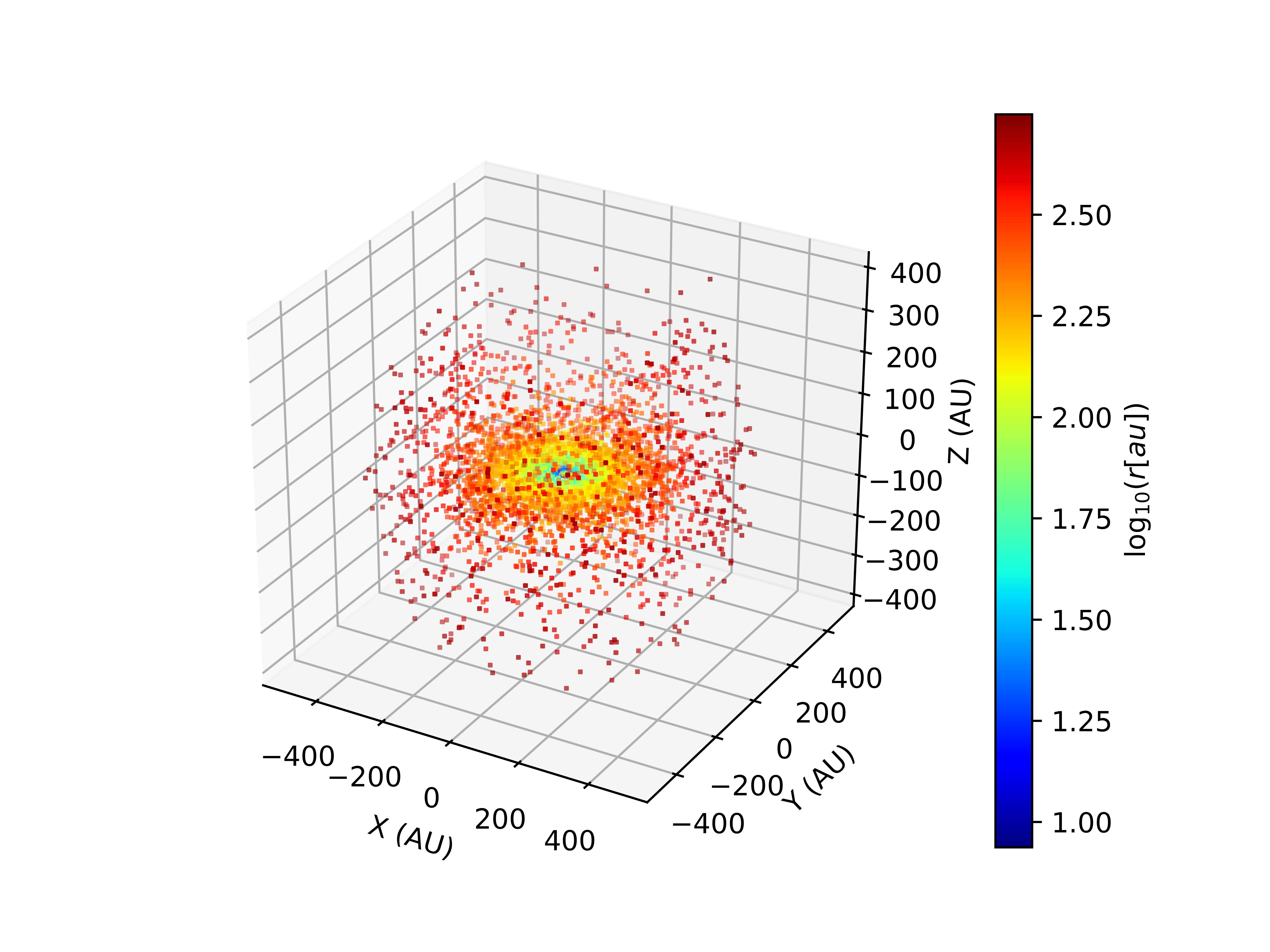
d. Plot the modelled region:
#-----------------------------------------------
#3D Points Distribution (weighting with density)
#-----------------------------------------------
tag = 'Main'
dens_plot = density.total / 1e6

weight = 10*Rho0
r = GRID.rRTP[0] / u.au #GRID.rRTP hosts [r, R, Theta, Phi] --> Polar GRID
Plot_model.scatter3D(GRID, density.total, weight,
                     NRand = 4000, colordim = r, axisunit = u.au,
                     cmap = 'jet', colorscale = 'log',
                     colorlabel = r'${\rm log}_{10}(r [au])$',
                     output = '3Dpoints%s.png'%tag, show = False)
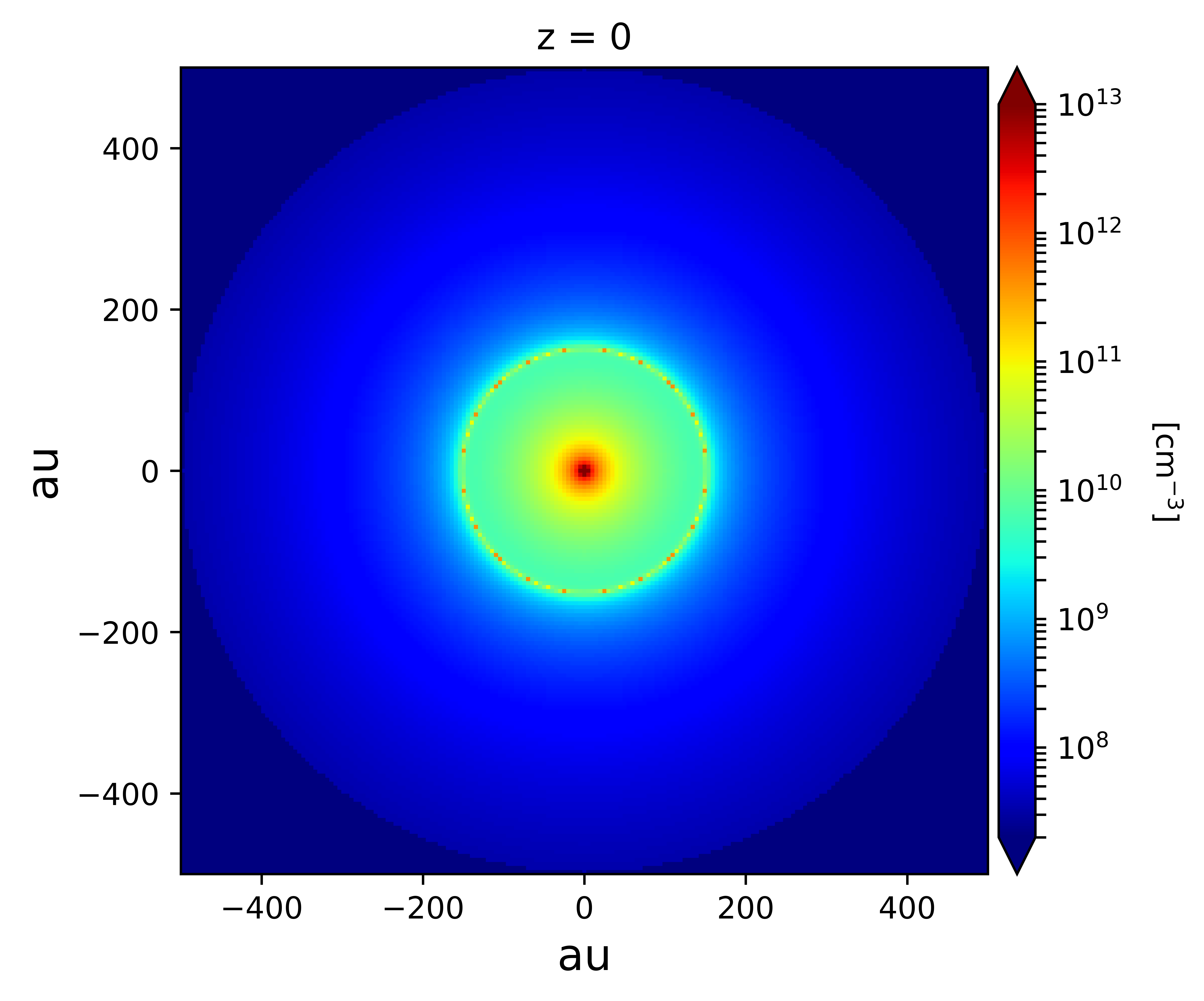
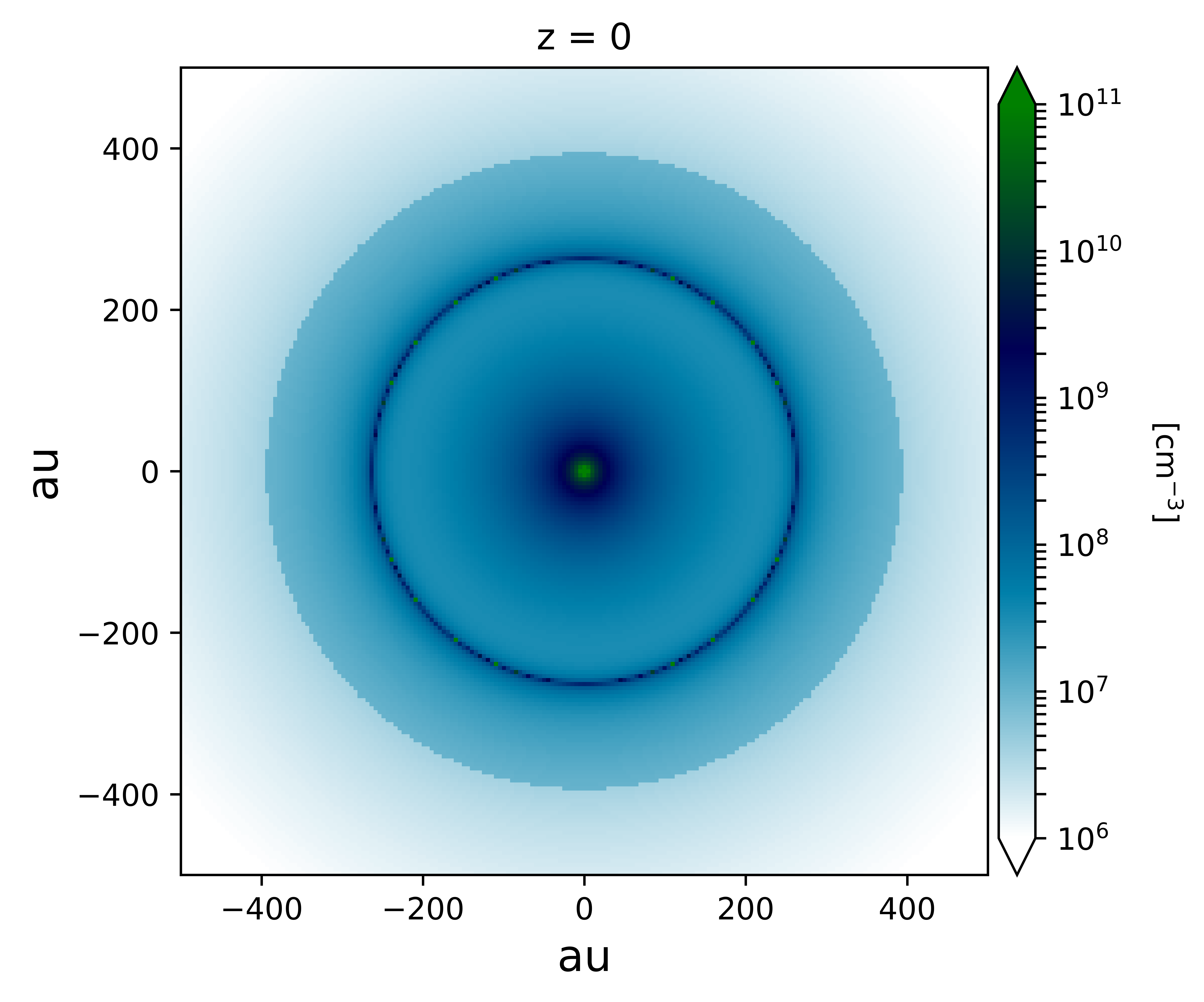
#---------------------
#2D PLOTTING (Density)
#---------------------

vmin, vmax = np.array([2e13, 1e19]) / 1e6
norm = colors.LogNorm(vmin=vmin, vmax=vmax)

Plot_model.plane2D(GRID, dens_plot, axisunit = u.au,
                   cmap = 'jet', plane = {'z': 0*u.au},
                   norm = norm, colorlabel = r'$[\rm cm^{-3}]$',
                   output = 'DensMidplane_%s.png'%tag, show = False)
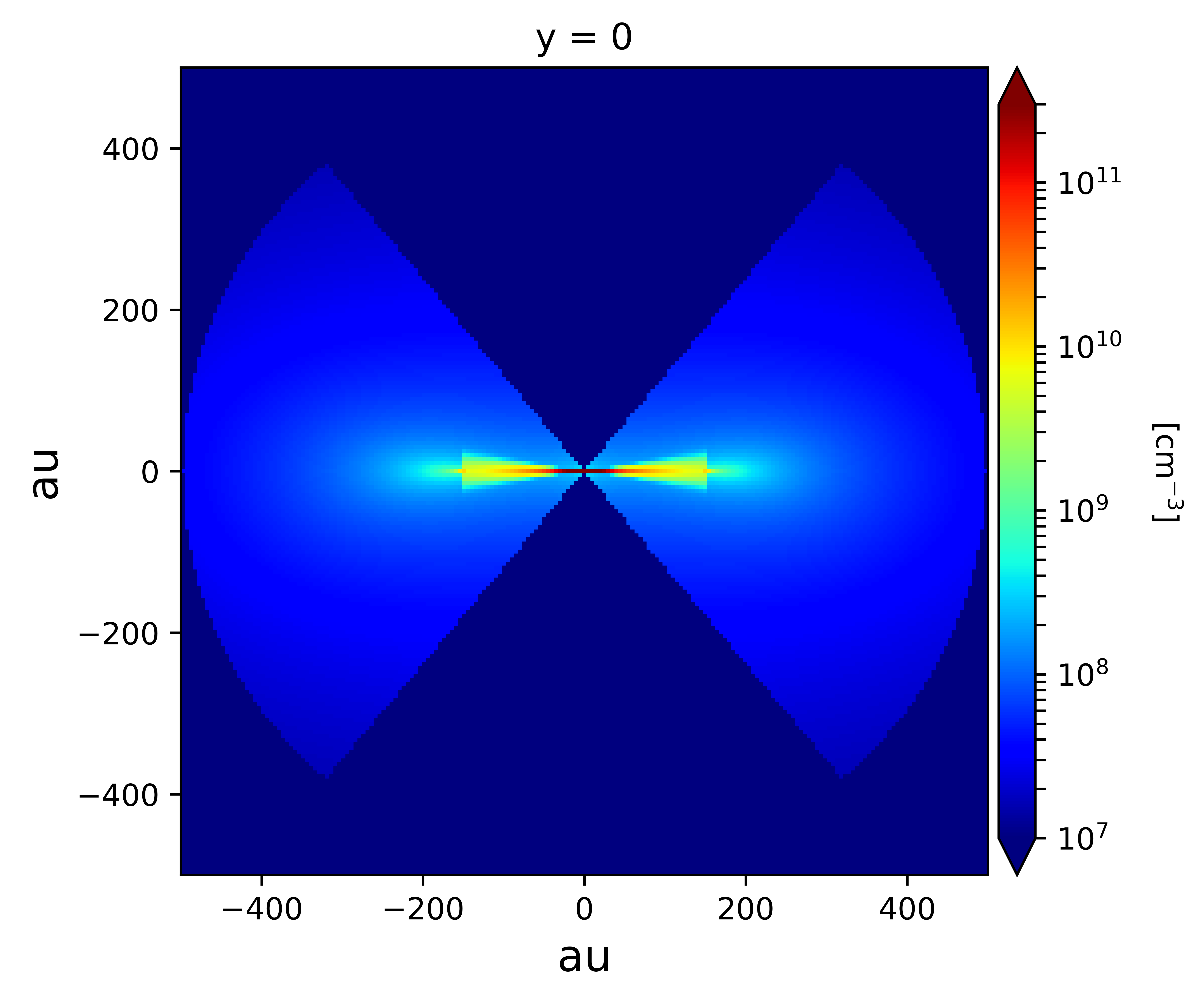
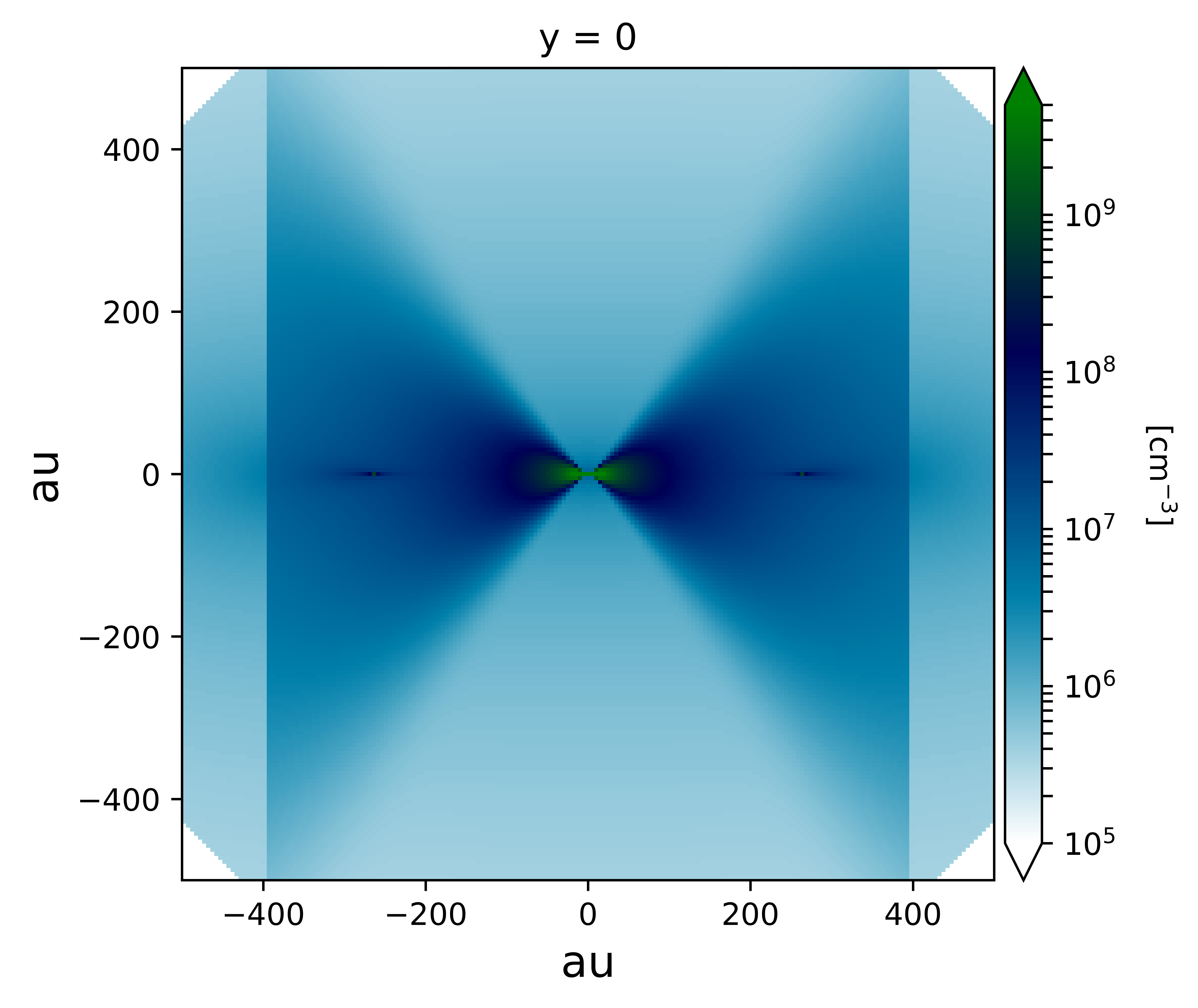
vmin, vmax = np.array([1e13, 3e17]) / 1e6
norm = colors.LogNorm(vmin=vmin, vmax=vmax)

Plot_model.plane2D(GRID, dens_plot, axisunit = u.au,
                   cmap = 'jet', plane = {'y': 0*u.au},
                   norm = norm, colorlabel = r'$[\rm cm^{-3}]$',
                   output = 'DensVertical_%s.png'%tag, show = False)
e. Write the numbers into a file, in this case readable in LIME:
#-----------------------------
#WRITING DATA for LIME
#-----------------------------
prop = {'dens_H2': density.total,
        'temp_gas': temperature.total,
        'vel_x': vel.x,
        'vel_y': vel.y,
        'vel_z': vel.z,
        'abundance': abundance,
        'gtdratio': gtdratio}
lime = rt.Lime(GRID)
lime.finalmodel(prop)
f. And print some useful information:
Model.PrintProperties(density, temperature, GRID)
print ('Ellapsed time: %.3fs' % (time.time() - t0)) #TIMING
Example 2
Source code and figures on GitHub: hamburger_standard
Note
Standard Hamburger: Class 0/I Young Stellar Object with self-obscuration in the (sub)mm spectral indices.
Model: Ulrich envelope + Hamburger disc.
Useful references: Lee+2017b, Li+2017, Galvan-Madrid+2018 (Submitted to ApJ)
The preamble: same as Example 1
a. The general parameters:
MStar = 0.86 * u.MSun
MRate = 5.e-6 * u.MSun_yr
RStar = u.RSun * ( MStar/u.MSun )**0.8
LStar = u.LSun * ( MStar/u.MSun )**4
TStar = u.TSun * ( (LStar/u.LSun) / (RStar/u.RSun)**2 )**0.25
Rd = 264. * u.au

print ('RStar:', RStar/u.RSun, ', LStar:', LStar/u.LSun, ', TStar:', TStar)
b. The grid:
#Cubic grid, each edge ranges [-500, 500] au.
sizex = sizey = sizez = 500 * u.au
Nx = Ny = Nz = 200 #Number of divisions for each axis
GRID = Model.grid([sizex, sizey, sizez], [Nx, Ny, Nz])
NPoints = GRID.NPoints #Number of nodes in the grid
c. The physical properties.
Note
The final density Structure should be defined by merging both the Envelope density and the Disc density (as shown in the following lines) since they were calculated separately from 2 different models.
#-------------
#DENSITY
#-------------

#--------
#ENVELOPE
#--------
Rho0 = Res.Rho0(MRate, Rd, MStar)
Arho = None
Renv = 2.5 * Rd
densEnv = Model.density_Env_Disc(RStar, Rd, Rho0, Arho, GRID,
                                 discFlag = False, envFlag = True,
                                 renv_max = Renv)
#-------
#DISC
#-------
H0sf = 0.03 #Disc scale height factor (H0 = H0sf * RStar)
Arho = 5.25 #Disc density factor
Rdisc = 1.5 * Rd
densDisc = Model.density_Hamburgers(RStar, H0sf, Rd, Rho0, Arho, GRID,
                                    discFlag = True,
                                    rdisc_max = Rdisc)
#---------------------
#The COMPOSITE DENSITY
#---------------------
density = Model.Struct( **{ 'total': densEnv.total + densDisc.total,
                            'disc': densDisc.total,
                            'env': densEnv.total,
                            'H': densDisc.H,
                            'Rt': densDisc.Rt,
                            'discFlag': True,
                            'envFlag': True,
                            'r_disc': densDisc.r_disc,
                            'r_env': densEnv.r_env,
                            'streamline': densEnv.streamline} )

#-----------
#TEMPERATURE
#-----------
T10Env = 250. #Envelope temperature at 10 au
Tmin = 10. #Minimum possible temperature. Every node with T<Tmin will inherit Tmin.
BT = 60. #Adjustable factor for disc temperature. Extra, or less, disc heating.
temperature = Model.temperature_Hamburgers(TStar, RStar, MStar, MRate, Rd,
                                           T10Env, BT, density, GRID,
                                           Tmin_disc = Tmin, inverted = False)

#--------
#VELOCITY
#--------
vel = Model.velocity(RStar, MStar, Rd, density, GRID)

#-------------------------------
#ABUNDANCE and GAS-to-DUST RATIO
#-------------------------------
ab0 = 5e-8 #CH3CN abundance vs H2
abundance = Model.abundance(ab0, NPoints)

gtd0 = 100. #Gas to dust ratio (H2 vs Dust)
gtdratio = Model.gastodust(gtd0, NPoints)
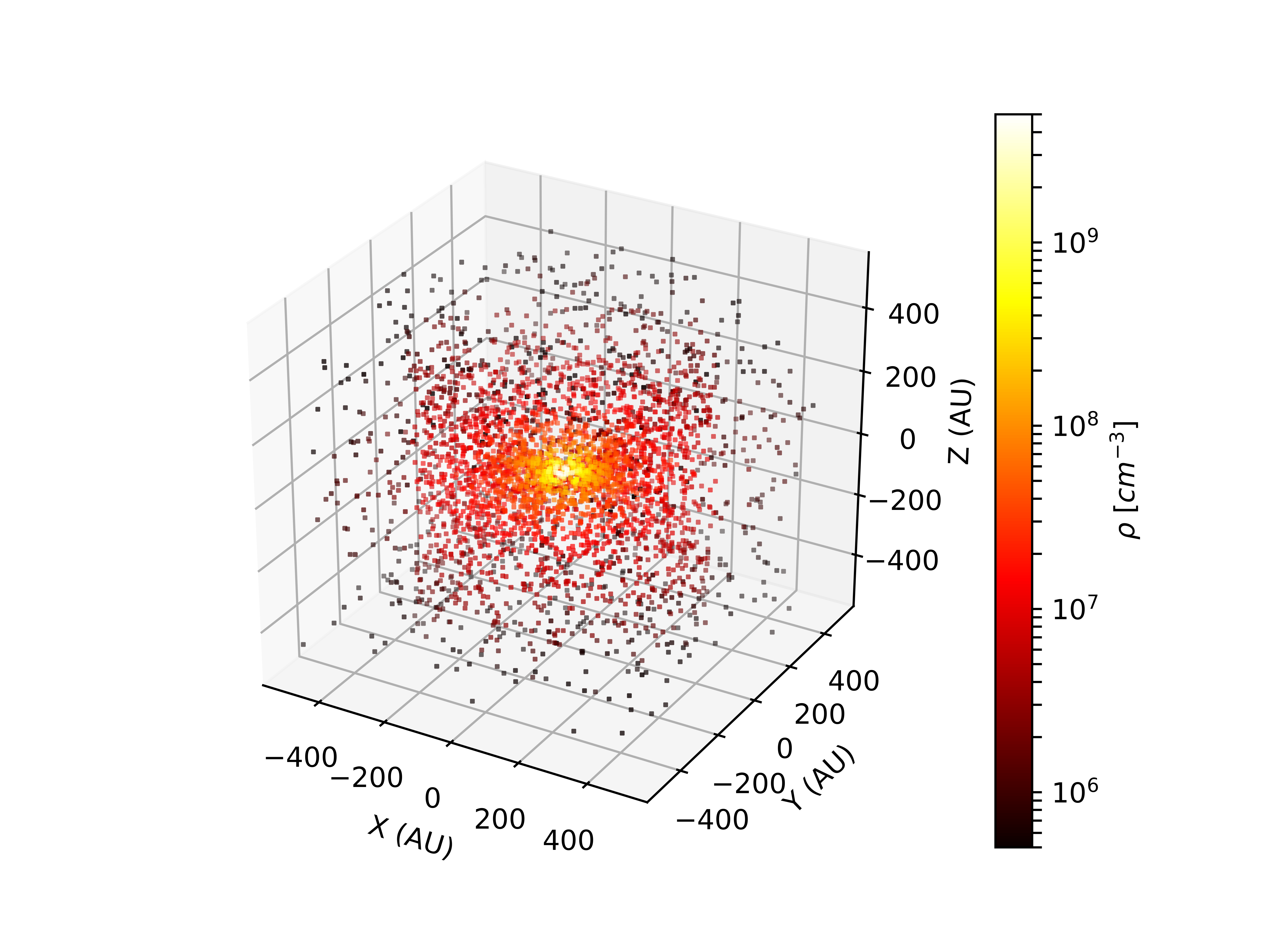
d. Plot the modelled region:
#----------------------------------------
#3D PLOTTING (weighting with temperature)
#----------------------------------------
tag = 'Burger'
dens_plot = density.total / 1e6

vmin, vmax = np.array([5e11, 5e15]) / 1e6
norm = colors.LogNorm(vmin=vmin, vmax=vmax)

weight = 10*T10Env
Plot_model.scatter3D(GRID, temperature.total, weight, NRand = 4000,
                     colordim = dens_plot, axisunit = u.au, cmap = 'hot',
                     norm = norm,
                     colorlabel = r'${\rm log}_{10}(\rho [cm^{-3}])$',
                     output = '3Dpoints%s.png'%tag, show = False)
#----------------------------------------
#2D PLOTTING (Density and Temperature)
#----------------------------------------

vmin, vmax = np.array([1e12, 1e17]) / 1e6
norm = colors.LogNorm(vmin=vmin, vmax=vmax)

Plot_model.plane2D(GRID, dens_plot, axisunit = u.au,
                   cmap = 'ocean_r', plane = {'z': 0*u.au},
                   norm = norm, colorlabel = r'$[\rm cm^{-3}]$',
                   output = 'DensMidplane_%s.png'%tag, show = False)
vmin, vmax = np.array([1e11, 5e15]) / 1e6
norm = colors.LogNorm(vmin=vmin, vmax=vmax)

Plot_model.plane2D(GRID, dens_plot, axisunit = u.au,
                   cmap = 'ocean_r', plane = {'y': 0*u.au},
                   norm = norm, colorlabel = r'$[\rm cm^{-3}]$',
                   output = 'DensVertical_%s.png'%tag, show = False)
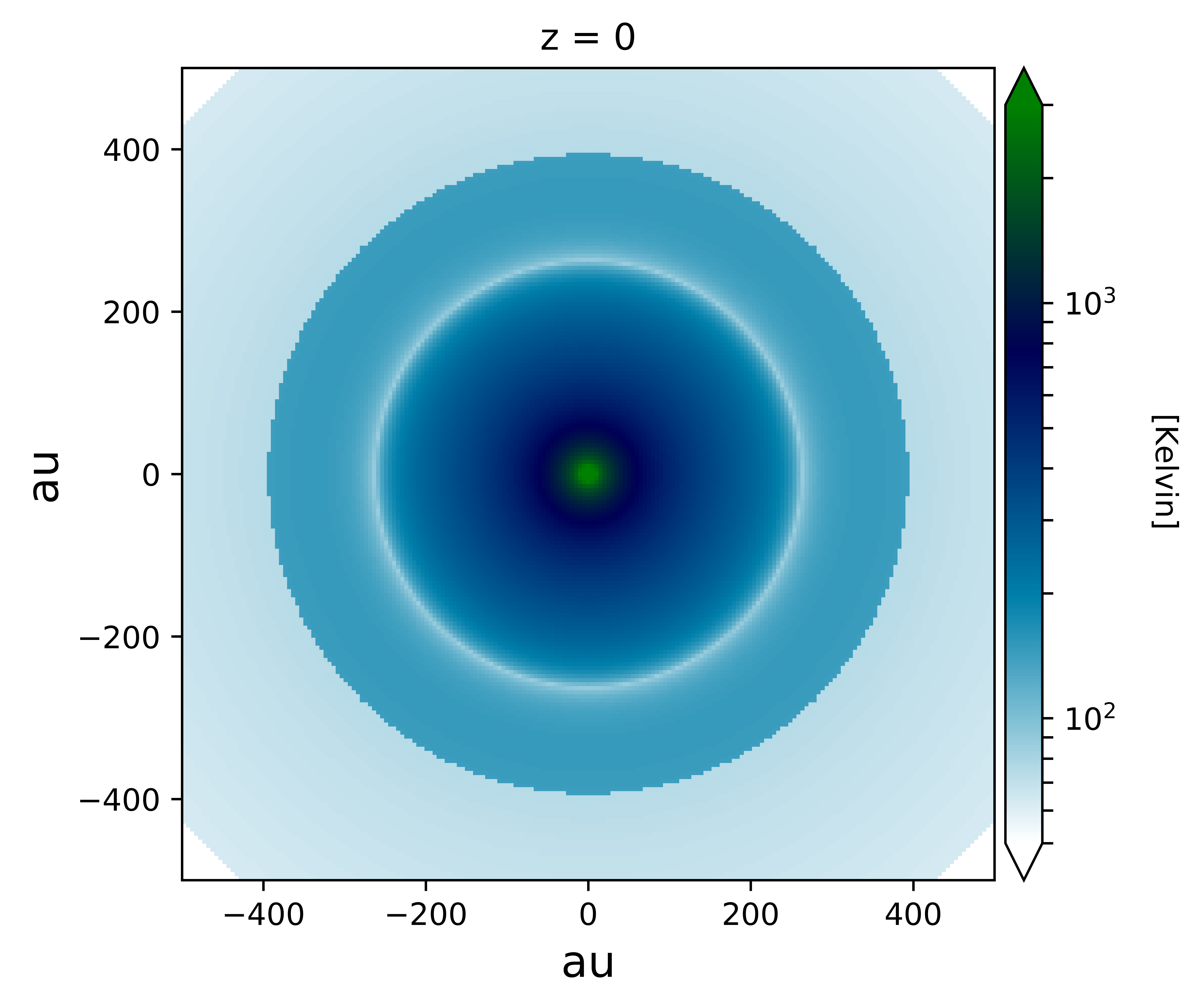
vmin, vmax = np.array([5e1, 3e3])
norm = colors.LogNorm(vmin=vmin, vmax=vmax)

Plot_model.plane2D(GRID, temperature.total, axisunit = u.au,
                   cmap = 'ocean_r', plane = {'z': 0*u.au},
                   norm = norm, colorlabel = r'[Kelvin]',
                   output = 'TempMidplane_%s.png'%tag, show = False)
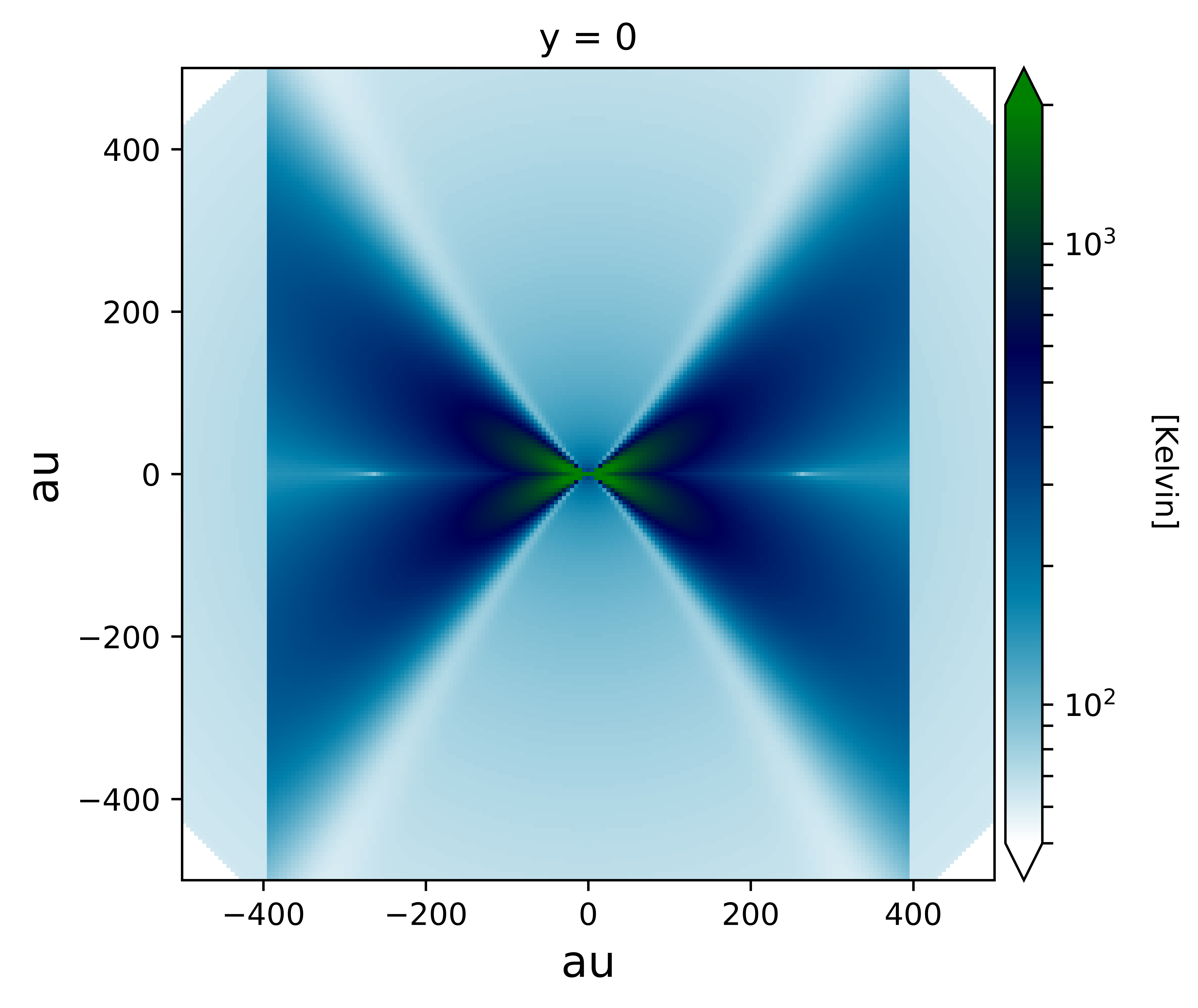
vmin, vmax = np.array([5e1, 2e3])
norm = colors.LogNorm(vmin=vmin, vmax=vmax)

Plot_model.plane2D(GRID, temperature.total, axisunit = u.au,
                   cmap = 'ocean_r', plane = {'y': 0*u.au},
                   norm = norm, colorlabel = r'[Kelvin]',
                   output = 'TempVertical_%s.png'%tag, show = False)
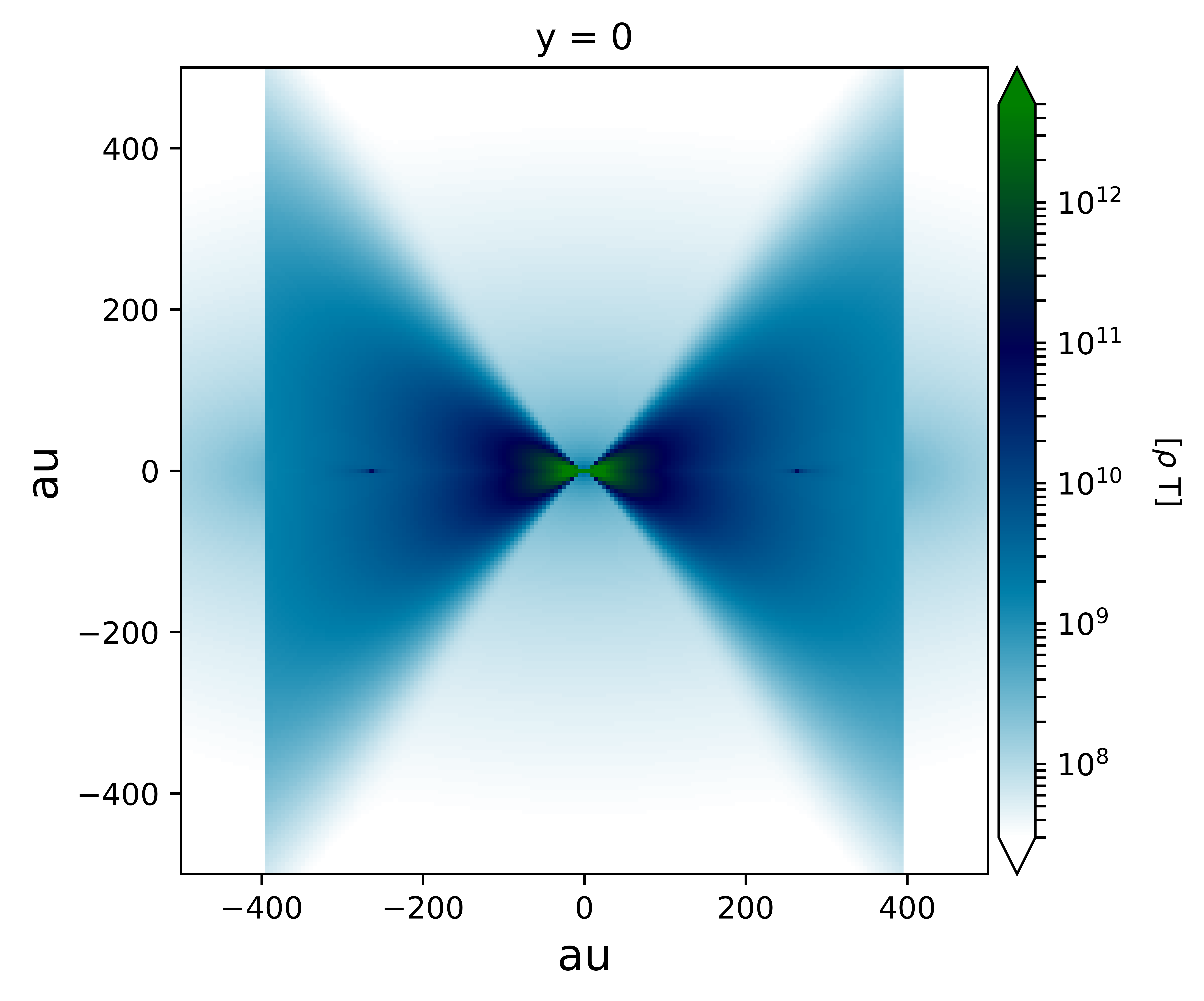
vmin, vmax = np.array([3e7, 5e12])
norm = colors.LogNorm(vmin=vmin, vmax=vmax)

Plot_model.plane2D(GRID, temperature.total * dens_plot, axisunit = u.au,
                   cmap = 'ocean_r', plane = {'y': 0*u.au},
                   norm = norm, colorlabel = r'[$\rho$ T]',
                   output = 'Emissivity_%s.png'%tag, show = False)
e. Write the data into a file:
#-----------------------------
#WRITING DATA for LIME
#-----------------------------
prop = {'dens_H2': density.total,
        'temp_gas': temperature.total,
        'vel_x': vel.x,
        'vel_y': vel.y,
        'vel_z': vel.z,
        'abundance': abundance,
        'gtdratio': gtdratio}
lime = rt.Lime(GRID)
lime.finalmodel(prop)

#-------------------------------------
#WRITING DATA into file in LIME format
#-------------------------------------
Model.DataTab_LIME(density.total, temperature.total, vel, abundance, gtdratio, GRID)
f. To finish, print some useful information:
Model.PrintProperties(density, temperature, GRID)
print ('Ellapsed time: %.3fs' % (time.time() - t0)) #TIMING