Modelling multiple star forming regions
Example 1
Source codes and figures on GitHub: two_sources
The first 2 examples of the section
Modelling a single star forming region
will be used here to illustrate how to overlap two (or more) models in a single global grid.
The overlaped physical properties are computed as in section 3.2 of Izquierdo+2018. See also Overlap.
Note
W33A MM1-Main: The most massive compact source of the complex star forming region W33A MM1.
Model: Ulrich envelope + Pringle disc.
Useful references: Galvan-Madrid+2010, Maud+2017, Izquierdo+2018
+
Standard Hamburger: Class 0/I Young Stellar Object with self-obscuration in the (sub)mm spectral indices.
Model: Ulrich envelope + Hamburger disc.
Useful references: Lee+2017b, Li+2017, Galvan-Madrid+2018 (Submitted to ApJ)
Warning
The execution codes for both compact sources are identical, except for the additions that are made explicit here. The following lines must be added after the definition of the Physical properties and for each compact source separately. Since we are going to overlap the models the writing-into-file process is slightly different (see below).
Additions for W33A MM1-Main
Since there is no longer an (isolated) single model, geometric changes may be required to better reproduce real scenarios. Let’s add some lines to account for the centering, inclination and systemic velocity of each modelled region.
#-------------------------
#ROTATION, VSYS, CENTERING
#-------------------------
xc, yc, zc = [-250*u.au, 350*u.au, 300*u.au]
CENTER = [xc, yc, zc] #New center of the region in the global grid
v_sys = 3320. #Systemic velocity (vz) of the region (in m/s)
newProperties = Model.ChangeGeometry(GRID, center = CENTER, vsys = v_sys,  vel = vel,
                                     rot_dict = { 'angles': [np.pi/4, 1.87*np.pi],
                                                  'axis': ['x','z'] })
The GRID and vel objects should inherit their new state hosted in
newProperties as a result of the geometric and shifting modifications.
GRID.XYZ = newProperties.newXYZ #Redefinition of the XYZ grid
vel.x, vel.y, vel.z = newProperties.newVEL
The 3D plot of the modelled region, shifted and rotated:
#------------------------------------
#3D PLOTTING (weighting with density)
#------------------------------------
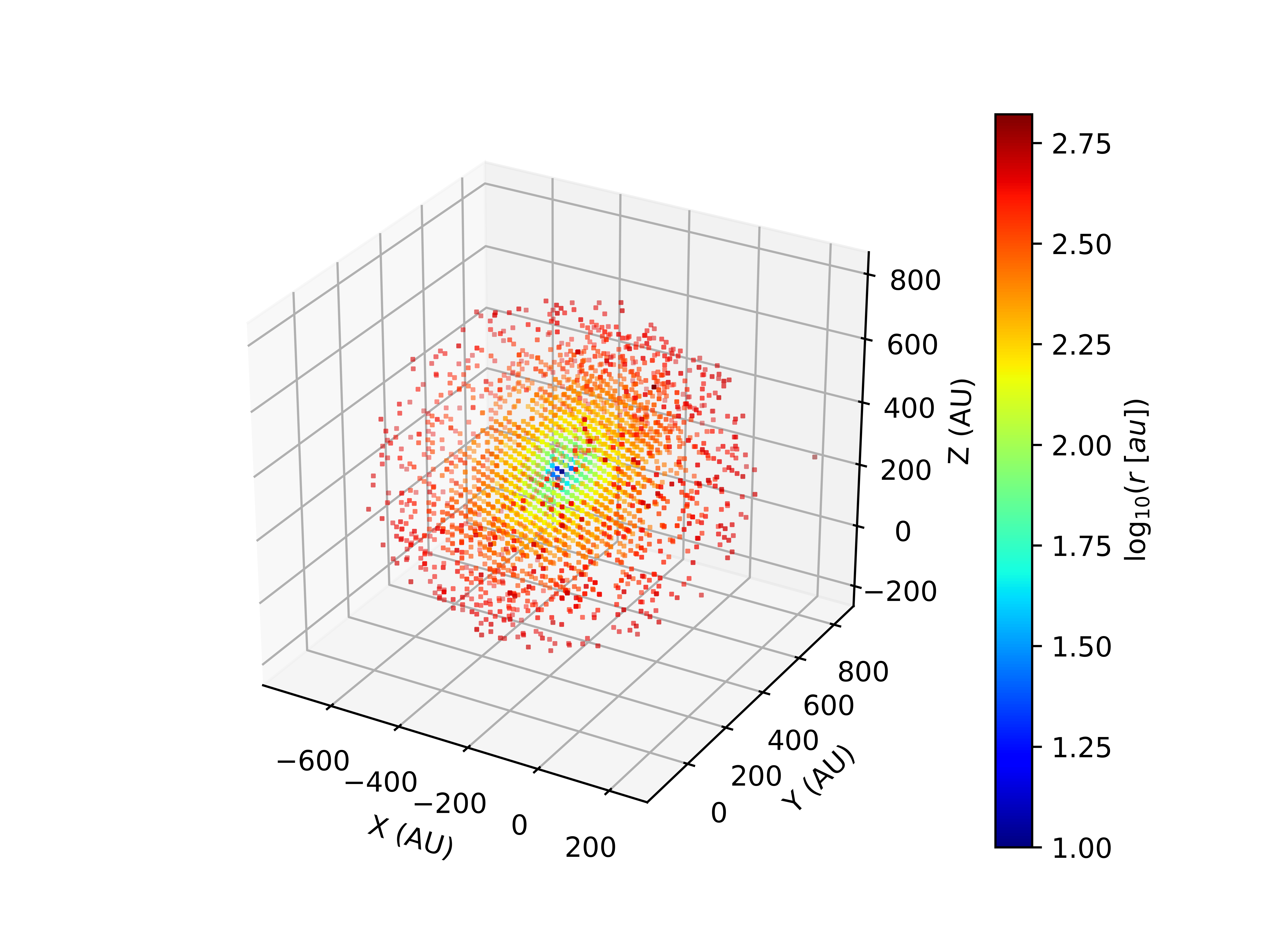
tag = 'Main'
weight = 10*Rho0
r = GRID.rRTP[0] / u.au #GRID.rRTP hosts [r, R, Theta, Phi] --> Polar GRID
Plot_model.scatter3D(GRID, density.total, weight,
NRand = 4000, colordim = r, axisunit = u.au,
cmap = 'jet', colorscale = 'log',
colorlabel = r'${\rm log}_{10}(r [au])$',
output = '3Dpoints%s.png'%tag, show = False)
Finally, the writing command. In this case it’s necessary to specify that the current model is actually a sub-model that will eventually be part of a global-model:
#-----------------------------
#WRITING DATA for LIME
#-----------------------------
tag = 'Main.dat'
prop = {'dens_H2': density.total,
        'temp_gas': temperature.total,
        'vel_x': vel.x,
        'vel_y': vel.y,
        'vel_z': vel.z,
        'abundance': abundance,
        'gtdratio': gtdratio}
lime = rt.Lime(GRID)
lime.submodel(prop, output=tag)
print('Output columns', lime.columns)
Note
When a sub-model is invoked, a new folder named Subgrids is created by default in the current working directory. All the sub-model data files are stored there for future use in the merging process.
Additions for the Hamburger
Similarly for the Hamburger model:
#-------------------------
#ROTATION, VSYS, CENTERING
#-------------------------
xc, yc, zc = [350*u.au, -150*u.au, -200*u.au]
CENTER = [xc, yc, zc] #Center of the region in the global grid
v_sys = -2000. #Systemic velocity (vz) of the region (in m/s)
newProperties = Model.ChangeGeometry(GRID, center = CENTER, vsys = v_sys,  vel = vel,
                                     rot_dict = { 'angles': [np.pi/2, np.pi/3],
                                                  'axis': ['y','z'] })

GRID.XYZ = newProperties.newXYZ #Redefinition of the XYZ grid
vel.x, vel.y, vel.z = newProperties.newVEL
The 3D plot of the modelled region, shifted and rotated:
#----------------------------------------
#3D PLOTTING (weighting with temperature)
#----------------------------------------
tag = 'Burger'
weight = 10*T10Env

vmin, vmax = np.array([5e11, 5e15]) / 1e6
norm = colors.LogNorm(vmin=vmin, vmax=vmax)

Plot_model.scatter3D(GRID, temperature.total, weight,
                     NRand = 4000, colordim = density.total / 1e6,
                     axisunit = u.au, cmap = 'jet', norm = norm,
                     colorlabel = r'${\rm log}_{10}(r [au])$',
                     output = '3Dpoints%s.png'%tag, show = False)
And the writing command:
#-----------------------------
#WRITING DATA for LIME
#-----------------------------
tag = 'Burger.dat'
prop = {'dens_H2': density.total,
        'temp_gas': temperature.total,
        'vel_x': vel.x,
        'vel_y': vel.y,
        'vel_z': vel.z,
        'abundance': abundance,
        'gtdratio': gtdratio}
lime = rt.Lime(GRID)
lime.submodel(prop, output=tag)
print('Output columns', lime.columns)
Overlapping the sub-models
Now that we have the data for each sub-model separately, we will invoke
the library BuildGlobalGrid to overlap them in a single global grid.
You can overlap all the sub-models available in the ./Subgrids folder,
or tell the module explicitly the list of sub-models to consider:
#------------------
#Import the package
#------------------
from sf3dmodels import Model, Plot_model as Pm
import sf3dmodels.utils.units as u
import sf3dmodels.rt as rt
from sf3dmodels.grid import Overlap
#-----------------
#Extra libraries
#-----------------
import numpy as np

#---------------
#DEFINE THE GRID
#---------------
sizex = sizey = sizez = 1000 * u.au
Nx = Ny = Nz = 120
GRID = Model.grid([sizex, sizey, sizez], [Nx, Ny, Nz])

#------------------
#INVOKE BGG LIBRARY
#------------------
columns = ['id', 'x', 'y', 'z', 'dens_H2', 'temp_gas', 'vel_x', 'vel_y', 'vel_z', 'abundance', 'gtdratio']
overlap = Overlap(GRID)
finalprop = overlap.fromfiles(columns, submodels = 'all')

"""Instead of picking all the submodels available in ./Subgrids you
can explicitly specify the ones that you want to overlap. The next two lines are equivalent to
the last one:

data2merge = ['Main.dat', 'Burger.dat']
finalprop = overlap.fromfiles(columns, submodels = data2merge)
"""
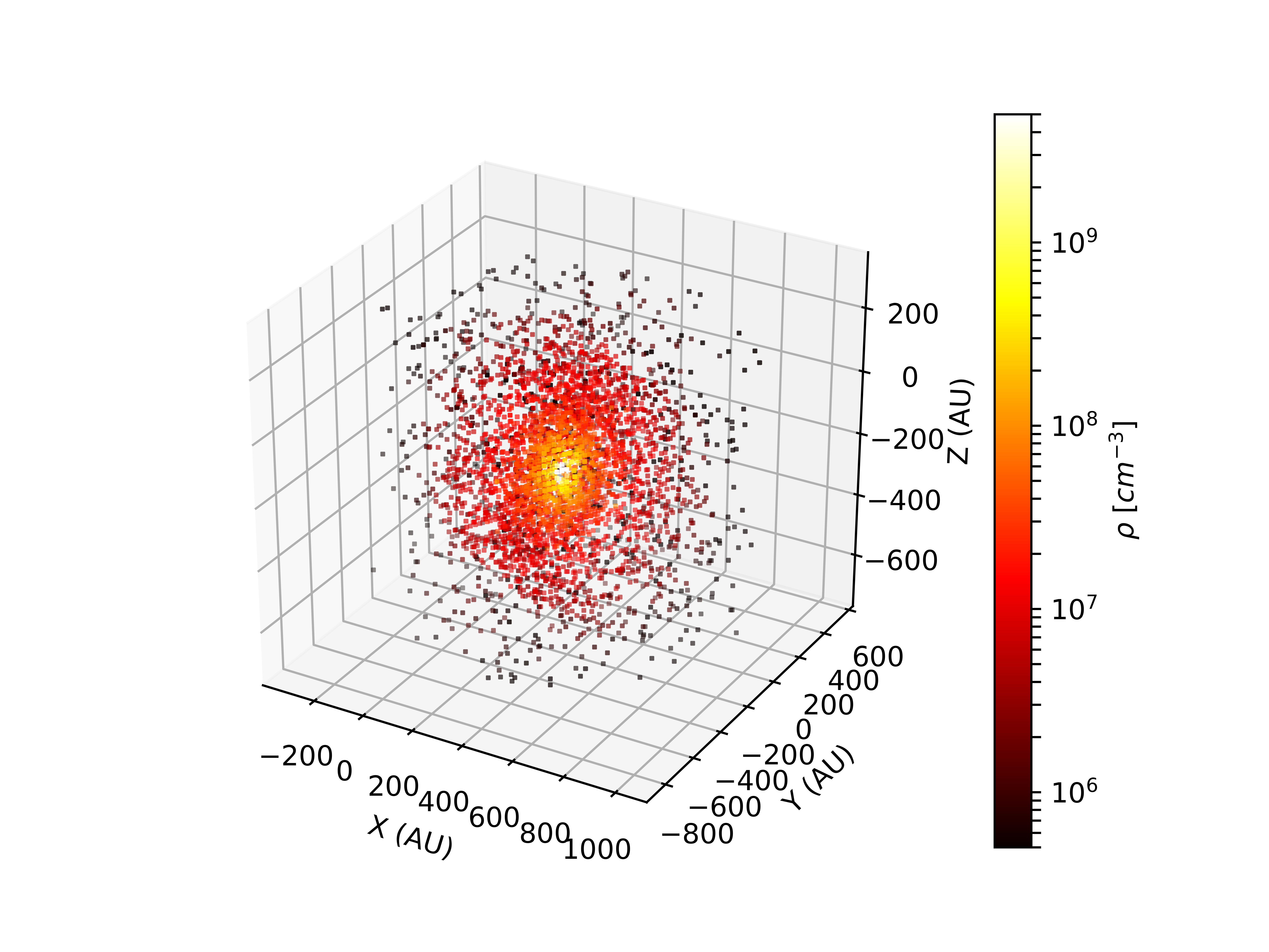
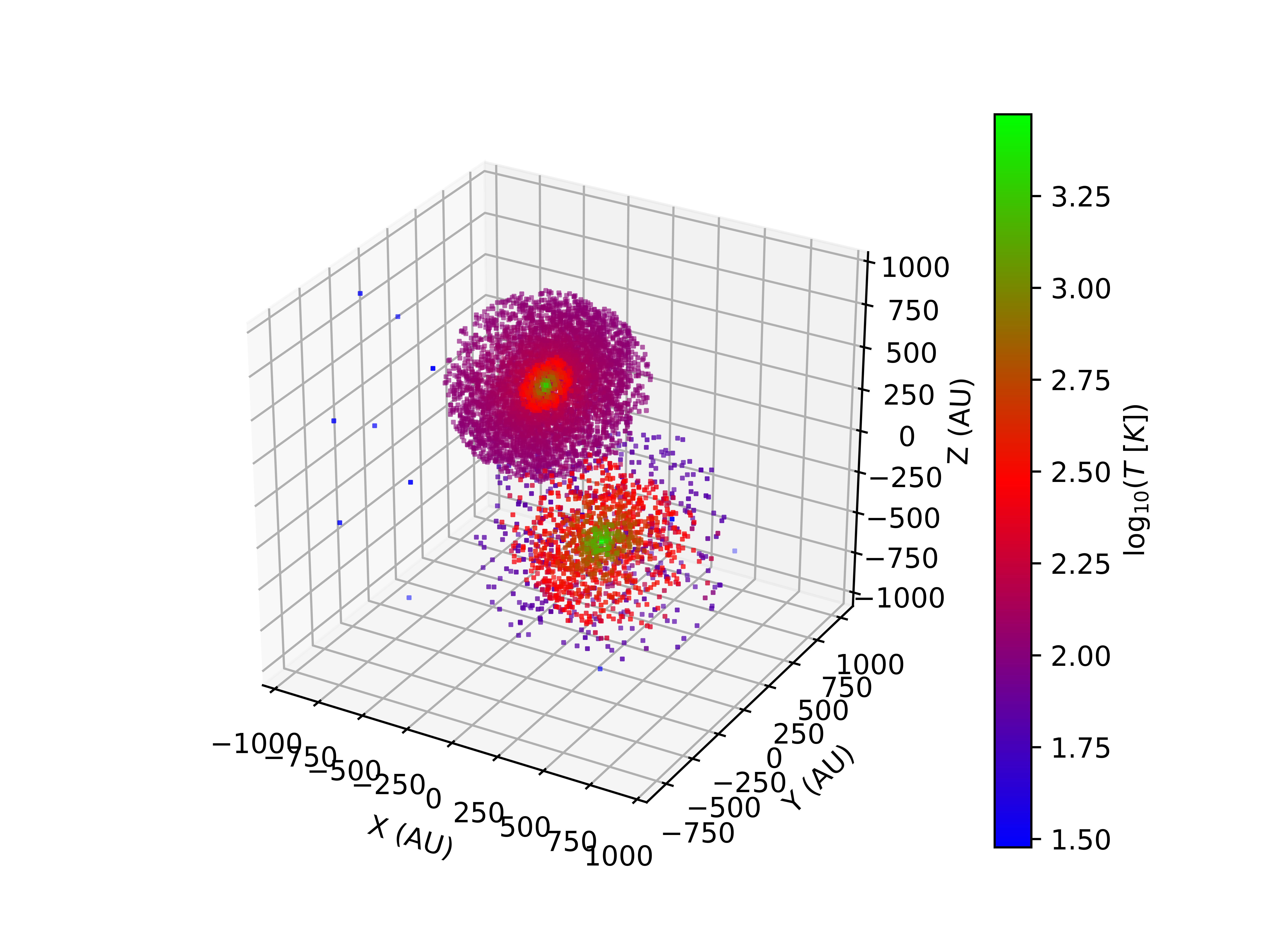
Plotting the result:
density = global_prop.density / 1e6 #cm^-3
temperature = global_prop.temperature

weight = 400 * np.mean(density)

#-----------------
#Plot for DENSITY
#-----------------
Pm.scatter3D(GRID, density, weight, NRand = 7000, axisunit = u.au,
             colorscale = 'log', cmap = 'hot',
             colorlabel = r'${\rm log}_{10}(\rho [cm^{-3}])$',
             output = 'global_grid_dens.png')

#--------------------
#Plot for TEMPERATURE
#--------------------
Pm.scatter3D(GRID, density, weight, colordim = temperature,
             NRand = 7000, axisunit = u.au, colorscale = 'log',
             cmap = 'brg', colorlabel = r'${\rm log}_{10}(T$ $[K])$',
             output = 'global_grid_temp.png')

Radiative Transfer with LIME
Dust continuum images